ECE298JA-F16
Concepts in Mathematics: ECE Webpage ECE298-JA; ECE-298JA; UIUC Course Explorer: ECE-298-JA; Time: 11-11:50 MWF; Location: 2013 ECEB (official); Register
- Professor: Jont B. Allen (jontalle@illinois.edu), TA: Sarah Robinson (srrobin2@illinois.edu)
- Syllabus: ECE298JA-F16; Flyer; Class notes: pdfBook (optional): Stillwell 3d edition, google for pdf, Video of Stillwell presentation, pdf, Boas;
- Exams: Exam I; Exam II; Exam III; About the final; Grades: statistics and distributions
- Office Hours (TA): Mon 12-1pm & Tues 4-5pm (Tues 5-6pm available by appointment) Location: 2137 Beckman (next to ECEB); Allen by apt.
- Extra TA Office Hours Fridays Oct 28, 12-1pm & Nov 4, 12-1pm in 2137 Beckman
- General interest: Timeline; fun read; luminaries; Math history: site1, site2; Mathematical Notation by topic, alpha-order, use of Functions and their History, Mathematical vignettes
- Tools: MATLAB, Octave, Latex
- This week's schedule
ECE 298JA Schedule (Fall 2016)
| L | W | D | Date | Lecture and Assignment |
| Part I: Number systems (10 Lectures) | ||||
| 1 | 1 34 | M | 8/22 | Introduction & Historical Overview; Lecture 0: pdf;
The Pythagorean Theorem & the Three streams: |
| 2 | W | 8/24 | Lecture: Number Systems (Stream 1) Taxonomy of Numbers, from Primes {$\pi_k$} to Complex {$\mathbb C$}: {$\pi_k \in \mathbb P \subset \mathbb N \subset \mathbb Z \subset \mathbb Z \cup \mathbb F = \mathbb Q \subset \mathbb Q \cup \mathbb I = \mathbb R \subset \mathbb C $} First use of zero as a number (Brahmagupta defines rules); First use of {$\infty $} (Bhaskara's interpretation) Floating point numbers IEEE 754 (c1985); History Read: Lec. 2 (pp. 24-29) | |
| 3 | F | 8/26 | Lecture: The role of physics in Mathematics: Math is a language, designed to do physics The Fundamental theorems of Mathematics: 1) Arithmetic (i.e., primes), 2) Algebra, 3) Calculus (& Set Theory) and other key concepts: History review: BC: Pythagoras; Aristotle; 17C: Mersenne; Galilei, Galileo; Hooke; Boyle; Newton; 18C: Bernoulli, Daniel; Euler; Lagrange; d'Alembert; 19C: Gauss; Laplace; Fourier; Von Helmholtz; Heaviside; Rayleigh; Read: Lec. 3 (pp. 29-32) | |
| 4 | 2 35 | M | 8/29 | Lecture: Two Prime Number Theorems: How to identify Primes (Brute force method: Sieve of Eratosthenes) 1) Fundamental Thm of Arith 2) Prime Number Theorem: Statement, Prime number Sieves Why are integers important?Public-private key systems (internet security) Elliptic curve RSA Pythagoras and the Beauty of integers: Integers {$\Leftrightarrow$} 1) Physics: The role of Acoustics & Electricity (e.g., light): 2) Eigenmodes: Mathematics in Music and acoustics: Strings, Chinese Bells, chimes; Read: Lec 4 (pp.32-33, 70-75); A short history of primes, History of PNT NS-1 Due Homework 2 (NS-2): Prime numbers, GCD, CFA; pdf, Due 9/7 |
| 5 | W | 8/31 | Lecture: Euclidean Algorithm for the GCD; Coprimes Definition of the {$k=\text{gcd}(m,n)$} with examples; Euclidean algorithm Properties and Derivation of GCD & Coprimes Algebraic Generalizations of the GCD Read: Lec. 5 (pp. 33, 73-75) | |
| 6 | F | 9/2 | Lecture: Continued Fraction algorithm (Euclid & Gauss, JS10, p. 47)
The Rational Approximations of irrational {$\sqrt{2} \approx 17/12\pm 0.25%)$} and transcendental {$(\pi \approx 22/7)$} numbers | |
| - | 3
36 | M | 9/5 | Labor Day Holiday -- No class |
| 7 | W | 9/7 | Lecture: Pythagorean triplets {a, b, c \in {\mathbb N}$} such that {$c^2=a^2+b^2$} Examples of PTs & Euclid's formula Properties, examples, History NS-2 Due Read: Lec. 7 (p. 36, 77-79) | |
| 8 | F | 9/9 | Lecture: Pell's Equation: General solution; Brahmagupta's solution by composition Chord and tangent solution (Diophantus {$\approx$}250CE) methods Read: Lec. 8 (pp. 36-37, 79-81) History of {$\mathbb R$} Optional: GCD Algorithm - Stillwell sections 3.3 & 5.3 | |
| 9 | 4 37 | M | 9/12 | Lecture: Fibbonacci Series Geometry & irrational numbers {$\sqrt{n}$} NS-3 Due Read: Lec 9 (pp. 37-38, 81-82) |
| 10 | W | 9/14 | Exam I (In Class): Number Systems |
| L | W | D | Date | Lecture and Assignment |
| Part II: Algebraic Equations (12 Lectures) | ||||
| 11 | F | 9/16 | Lecture: Analytic geometry as physics (Stream 2) The first "algebra" al-Khwarizmi (830CE) Polynomials, Analytic functions, {$\infty$} Series: Geometric {$\frac{1}{1-z}=\sum_{0}^\infty z^n$}, {$e^z=\sum_{0}^\infty \frac{z^n}{n!}$}; Taylor series; ROC; expansion point Read: Lec 11 | |
| 12 | 5 38 | M | 9/19 | Lecture: Complex analytic functions; Physical equations in several variables Summarize Lec 11:Detailed review of series representations of analytic functions: Poles, residues, ROC, etc. Geometry + Algebra {$\Rightarrow$} Analytic Geometry: From Euclid to Descartes+Newton Newton (1667) labels complex cubic roots as "impossible." Bombelli (1572) first uses complex numbers (JS10: p. 277-278) Read: Lec 12 Homework 4 (AE-1): Polynomials & Analytic functions and their inverse, Convolution, Newton's method (pdf, Due 9/28) |
| 13 | W | 9/21 | Lecture: Root classification for polynomials by convolution; Residue expansion Chinese discover Gaussian elimination (Jiuzhang suanshu) (JS10: p. 89) Gaussian elimination in one & two variables Solution of the quadratic (Brahmagupta, 628), cubic (c1545), quartic (Tartaglia et al..., 1535), quintic cannot be solved (Abel, 1826) Composition of polynomial equations (Bezout's Thm) Read: Lec 13 | |
| 14 | F | 9/23 | Lecture: Analytic Geometry (Fermat 1629; Descartes 1637) Descartes' insight: Composition of two polynomials of degrees: ({$m$}, {$n$} {$\rightarrow$} one of degree {$n\cdot m$}) Composition, elimination vs. intersection of polynomials: What is the difference? Detailed comparison of Euclid's Geometry (300BCE) and Algebra (830CE) Computing and interpreting the roots of the characteristic polynomial (CP) Linear equations are Hyperplanes in {$N$} dimensional space; 2 planes compose a line, 3 planes compose to a point Vectors, Complex planes & lines, Dot and cross products of vectors Read: Lec 14 | |
| 15 | 6 39 | M | 9/26 | Lecture: Gaussian elimination (intersection); Pivot matrices {$(\Pi_n)$}: {$U = \Pi_n^N P_n A$} gives upper-diagional {$U$} Read: Lec 15 Homework 5 (AE-2): Non-linear and linear systems of equations; Gaussian elimination; pdf Due 10/5 |
| 16 | W | 9/28 | Lecture: Composition of polynomials, ABCD matrix method ABCD Composition relations of transmission lines Read Lec 16 AE-1 Due | |
| 17 | F | 9/30 | Lecture: Introduction to the Riemann sphere (1851); (the extended plane) (JS10, p. 298-312) Mobius Transformation (youtube, HiRes), pdf description Understanding {$\infty$} by closing the complex plane; Chords on the sphere pdf Mobius transformations in matrix format Read: Lec. 17 | |
| 18 | 7 40 | M | 10/3 | Lecture: Fundamental Thm of Algebra (pdf) & Colorized plots Software: Matlab: zviz.zip, python |
| 19 | W | 10/5 | Lecture: Fourier Transforms for signals AE-2 Due Read: Lec 19; Fourier Transform (wikipedia), Notes on the Fourier series and transform from ECE 310 (including tables of transforms and derivations of transform properties) | |
| 20 | F | 10/7 | Lecture: Laplace transforms for systems The importance of Causality Cauchy Riemann role in the acceptance of complex functions: Convolution of the step function: {$u(t) \leftrightarrow 1/s$} vs. {$2\tilde{u}(t) \equiv 1+ \mbox{sgn}(t) \leftrightarrow 2\pi \delta(\omega) + 2/j\omega$} Read: Lec 20; Laplace Transform,Table of transforms | |
| 21 | 8 41 | M | 10/10 | Lecture: The nine postulates of Systems (aka, Network) pdf The important role of the Laplace transform re impedance: {$z(t) \leftrightarrow Z(s)$} A.E. Kennelly introduces complex impedance, 1893 pdf Fundamental limits of the Fourier re the Laplace Transform: {$\tilde{u}(t)$} vs. {$u(t)$} |
| 22 | W | 10/12 | No class due to Exam II: 7-10 PM; 2013 ECEB |
| L | W | D | Date | Lecture and Assignment |
| Part III: Scaler Differential Equations (12 Lectures) | ||||
| 23 | F | 10/14 | Lecture: Integration in the complex plane: FTC vs. FTCC Analytic vs complex analytic functions and Taylor formula Calculus of the complex {$s$} plane ({$s=\sigma+j\omega$}): {$dF(s)/ds$}, {$\int F(s) ds$} (Boas, see page 8) The convergent analytic power series: Region of convergence (ROC) Complex-analytic series representations: (1 vs. 2 sided); ROC of {$1/(1-s), 1/(1-x^2), -\ln(1-s)$} 1) Series; 2) Residues; 3) pole-zeros; 4) Continued fractions; 5) Analytic properties History: The amazing Bernoulli family; Fluid mechanics; airplane wings; natural logarithms Beginnings of modern mathematics: Euler and Bernoulli, Euler's standard circular-function package (Logs, exponentials, sin/cos) Inversion of analytic functions: Example: {$\tan^{-1}(z) = \frac{1}{2i}\ln \frac{i-z}{i+z}$}, the inverse of Euler's formula (1728) (Stillwell p. 314) Read: Lec 23 Homework 7 (DE-1): Series, differentiation, CR conditions, Bi-Harmonic functions: pdf, Due 10/24/2016 | |
| 24 | 9 42 | M | 10/17 | Lecture: Cauchy-Riemann (CR) conditions Cauchy-Riemann conditions and differentiation wrt {$s$}: {$Z^\prime(s) \equiv \frac{dZ(s)}{ds} = \frac{dZ(s)}{d\sigma} = \frac{dZ(s)}{dj\omega}$} Differentiation independent of direction in {$s$} plane: {$Z(s)$} obeys CR conditions: {$\frac{\partial R(\sigma,\omega)}{\partial\sigma} = \frac{\partial X(\sigma,\omega)}{\partial\omega}$} and {$\frac{\partial R(\sigma,\omega)}{\partial\omega} = -\frac{\partial X(\sigma,\omega)}{\partial\sigma}$} Cauchy-Riemann conditions require that Real and Imag parts of {$Z(s) = R(\sigma,\omega) + j X(\sigma,\omega)$} obey Laplace's Equation: {$\nabla^2 R=0$}, namely: {$\frac{\partial^2R(\sigma,\omega)}{\partial^2\sigma} + \frac{\partial^2 R(\sigma,\omega)}{\partial^2 \omega} =0 $} {$\nabla^2 X=0$}, namely: {$\frac{\partial^2 X(\sigma,\omega)}{\partial^2\sigma} + \frac{\partial^2 X(\sigma,\omega)}{\partial^2 \omega} =0$}, Biharmonic grid (zviz.m) Discussion of the solution of Laplace's equation given boundary conditions (conservative vector fields) Read: Lec 24 & Boas pages 13-26; Derivatives; Convergence and Power series |
| 25 | W | 10/19 | Lecture: Complex analytic functions and Brune impedance Complex impedance functions {$Z(s)$}, {$\Re Z(\sigma>0) \ge 0$}, Simple poles and zeros & 9 Postulates Time-domain impedance {$z(t) \leftrightarrow Z(s)$} Read: Lec 25 | |
| 26 | F | 10/21 | Lecture: Review session on multi-valued functions and complex integration Riemann sheets, colorized plots, branch cuts, Review of Fundamental Theorems of complex analytic functions. Laplace's equation and its role in Engineering Physics. What is the difference between a mass and an inductor? nonlinear elements; Examples of systems and the Nine postulates of systems. Homework 8 (DE-2): Inverse Laplace Transforms; Residue integration: pdf, Due 10/31/2016 | |
| 27 | M | 10/24 | Lecture: Three complex integration Theorems: Part I 1) Cauchy's Integral Theorem: {$\oint f(z) dz =0$} (Boas p. 45) vs. 2D Green's Thm (p. 49); Stokes (Thm, Bio) Read: Lec 27 & Boas p. 33-43 Complex Integration; Cauchy's Theorem DE-1 due | |
| 28 | W | 10/26 | Lecture: Three complex integration Theorems: Part II 2) Cauchy's Integral Formula: {$\frac{1}{2\pi j} \displaystyle \oint_{{\partial}_{\gamma}} \frac{f(z)}{z-z_0}dz = f(z_0) \, U(\gamma) \equiv 0$} if {$z_0 \notin \gamma^\circ$} 3) Cauchy's Residue Theorem Example by brute force integration: {$\oint_{|s|=1} \frac{ds}{s}= 2\pi j$} Read: Lec 28 & Boas p. 33-43 Complex Integration; Cauchy's Theorem | |
| 29 | F | 10/28 | Lecture: The Inverse Laplace Transform (ILT); poles and the Residue expansion: The case for causality {$t\le0$} Cauchy's Residue theorem {$\Leftrightarrow$} 2D Green's Thm (in {$\mathbb C$}) Homework 9 (DE-3): pdf, Due 11/7/2016 Read: Lec 29 | |
| 30 | 11 44 | M | 10/31 | Lecture: Inverse Laplace Transform: Use of the Residue theorem {$t>0$} Case for causality: Closing the contour: ROC as a function of {$e^{st}$}. Examples: {$F(s)=1 \leftrightarrow \delta(t)$} and {$u(t) \leftrightarrow 1/s$} Case of RC impedance {$ z(t) = R\delta(t)+u(t)/C \leftrightarrow R+1/sC $} RC admittance {$ y(t) = e^{-t}u(t) \leftrightarrow 1/(s+1) $} Semi-capacitor: {$ u(t)/\sqrt{t} \leftrightarrow \sqrt{\pi/s} $} Read: Lec 30 |
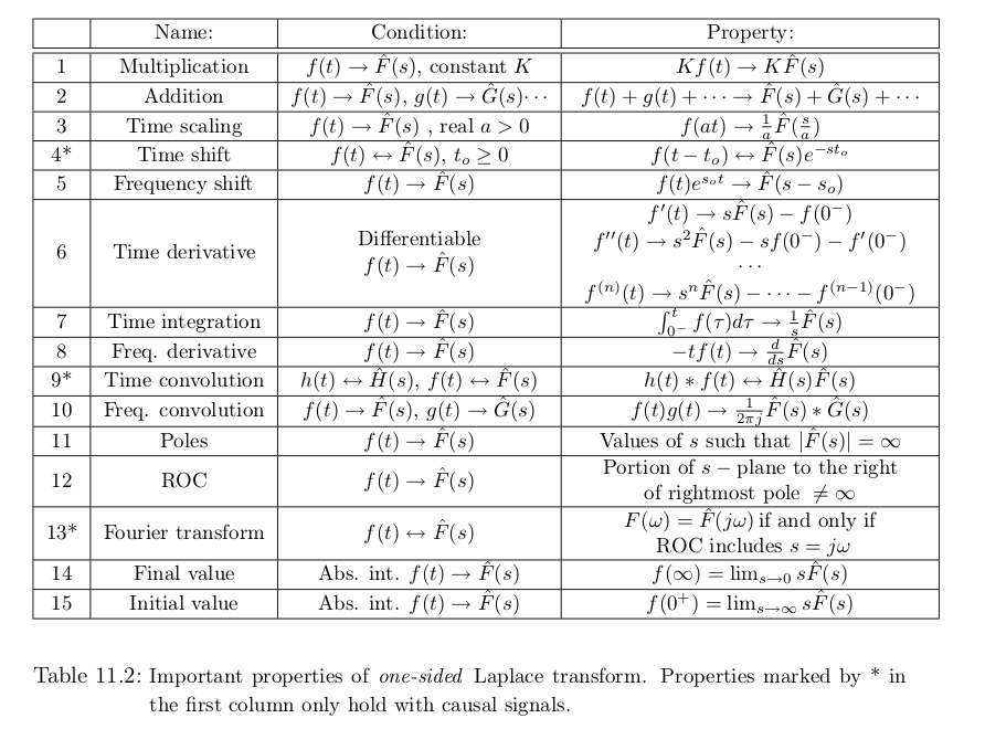
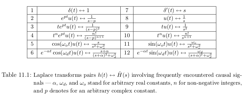
| 31 | W | 11/2 | Lecture: General properties of Laplace Transforms: Modulation, Translation, Convolution, periodic functions, etc. (png) Table of common LT pairs (png) Read: Lec 31 | |
| 32 | F | 11/4 | Lecture: General properties of Impedance (Z) and Transmission (ABCD) functions: Impedance {$Z(s) = V(s)/I(s) \rightarrow $} Generalized impedance and interesting story Raoul Bott Minimum phase impedance {$\rightarrow$} Simple poles & zeros in LHP ({$\sigma \le 0$}) Transfer {$H(s)=V_2/V_1, I_2/I_1 \rightarrow $} Allpass: {$|e^{-\jmath\phi(\omega)}|=1 \rightarrow$} poles in LHP, zeros in RHP Wiener's factorization theorem: {$H(s) = M(s)A(s)$} with factors Minimum phase {$M(s)$} & Allpass {$A(s)$} Read: Lec 32 | |
| 33 | 12 45 | M | 11/7 | Lecture: Riemann Zeta function {$\zeta(s)=\sum \frac{1}{n^s}$} Euler's vs. Riemann's Zeta Function (i.e., poles at the primes), music of primes, Analytic continuation, Tao Introduction to the Riemann zeta function (Stillwell p. 184) Euler's product formula; plot of Riemann-Zeta function showing magnitude and phase separately Inverse Laplace transform of {$\zeta(s) \leftrightarrow \mbox{Zeta}(t)$} DE-3 Due |
| 34 | W | 11/9 | No class due to Exam III: Thursday | |
| 34 | R | 11/10 | Exam III 7-10 PM; NOTE ROOM CHANGE: 2015ECEB |
| L | W | D | Date | Lecture and Assignment |
| Part IV: Vector (Partial) Differential Equations (9 Lectures) | ||||
| 35 | F | 11/11 | Lecture: Scaler wave equation {$\nabla^2 p = \frac{1}{c^2} \ddot{p}$} with {$c=\sqrt{ \eta P_o/\rho_o }$} Newton's formula: {$c=\sqrt{P_o/\rho_o}$} with an error of {$\sqrt{1.4}$} What Newton missed: Adiabatic compression {$PV^\eta=$} const with {$\eta = \frac{c_p}{c_v} = \frac{dof+2}{dof}=\frac{7}{5}$} d'Alembert solution: {$\psi = F(x-ct) + G(x+ct)$} Homework 10 (VC-1): pdf, Due: Nov 28 Mon (Alt 30 Wed) Read: Class Notes p. 1-2 | |
| 36 | 13 46 | M | 11/14 | Lecture: The Webster Horn Equation {$ \frac{1}{A(x)}\frac{\partial}{\partial x}A(x)\frac{\partial}{\partial x}{\cal P}(x,\omega) = \frac{s^2}{c^2}{\cal P}(x,\omega) $} Dot and cross product of vectors (repeat of Lec 14): {$ \mathbf{A} \!\cdot\! \mathbf{B}, \mathbf{A} \!\times\! \mathbf{B} $} vs. {$ \nabla \phi, \nabla\!\cdot\!\mathbf{B}, \nabla \!\times\! \mathbf{B} $} Curl examples Read: Class Notes p.3-10? |
| 37 | W | 11/16 | Lecture: Gradient, divergence, curl, scalar Laplacian and Vector Laplacian Gradient {$\nabla p(x,y,z)$}, divergence {$\nabla \cdot \mathbf{D}$} and Curl {$\nabla \times \mathbf{A}(x,y,z)$}, Scalar Laplacian {$\nabla^2 \phi$}, Vector Laplacian {$\nabla^2 \mathbf{E}$} Read: Lec 37 | |
| 38 | F | 11/18 | Lecture: More on the curl and divergence: Stokes' (curl) and Gauss' (divergence) Theorems, Vector Laplacian Homework 11 (VC-2): pdf, Due: Dec 7 Wed Read: Lec 38 | |
| - | 47 | Sa | 11/19 | Thanksgiving Holiday (11/19-11/27) |
| 39 | 14 48 | M | 11/28 | Lecture: J.C. Maxwell unifies Electricity and Magnetism (1861); Basic definitions: {$ \mathbf{E}, \mathbf{H}, \mathbf{B}, \mathbf{D} $}; O. Heaviside's (1884) vector form of Maxwell's Eqs.: {$\nabla \times \mathbf{E} = - \dot{\mathbf{B}} $} & {$\nabla \times \mathbf{H} = \dot{ \mathbf{D} }$} Differential and integral forms of Maxwell's Eqs. How a loudspeaker works: {$ \mathbf{F} = \mathbf{J} \times \mathbf{B} $} and EM Reciprocity; Magnetic loop video, citation VC-1 due Read: Lec 39 |
| 40 | W | 11/30 | Lecture: The Fundamental theorem of vector calculus: {$\mathbf{F}(x,y,z) = -\nabla{\phi(x,y,z)} + \nabla \times \mathbf{A}(x,y,z)$}, Definitions of Incompressable and irrotational fluids depend on two null-vector identities: DoC: {$\nabla\cdot\nabla\times(\text{vector})=0$} & CoG: {$\nabla\times\nabla(\text{scalar}) =0$}. Definition of the Conservative vector fields. Read: Lec 40 | |
| 41 | F | 12/2 | Lecture: The low-frequency quasi-static approximation: i.e., {$a < \lambda=c/f$} or {$f < c/a$}) are used for: Brune's Impedance ({$a \ll \lambda$}), Kirchhoff's Laws, the telegraph wave equation starting from Maxwell's equations. Impedance boundary conditions and generalized impedance: {$Z(s)\equiv \frac{\cal P}{\cal V} = r_0 \frac{1+\Gamma(s)}{1-\Gamma(s)}$} where {$ \Gamma(s) \equiv {\cal P}_-/{\cal P}_+ $} and {$r_0 = {\cal P_+}/{\cal V_+}$}, with {${\cal P}= {\cal P}_+ +{\cal P}_-$} and {${\cal V}= {\cal V}_+ -{\cal V}_-$}. Read: Lec 41 | |
| 42 | 15 49 | M | 12/5 | Lecture: Review The Fundamental Thms of Mathematics & their applications Theorems of Mathematics; Fundamental Thms of Mathematics (Ch. 9) Normal modes vs. eigen-states, delay and quasi-statics; The Hydrogen atom is an exponential horn: it is a waveguide with radial normal modes (eigen-states), occupied with electrons (EM energy), which escapes (i.e., radiates) as photons (free particles). This explains {$E=h\nu$}. Read: Lec 42 |
| 43 | W | 12/7 | Last day of Class: The ``quantum'' in QM refers to normal modes. Quantum mechanics is quasi-static, which assumes no delay. {$\Rightarrow$} Let {$c$}=speed of light; {$v$}=frequency; {$V$}=group-velocity, then {$E=h \nu$}, {$p=h/\lambda$} {$\rightarrow$} {$\nu = E/h, \lambda=h/p \rightarrow c = \lambda \nu = E/p$} (pdf) | |
| - | R | 12/8 | Reading Day | |
| - | M | 12/12 | Final Exam Monday Dec 12, 7-10pm ECEB 2013 |
Powered by PmWiki